Workflows

BT LITE

In case you want to explore gene expression across different datasets via a comparative visalization, BT LITE is a good starting point. It mainly allows you to visualize your data via

1. a heatmap showing general dataset coverage across brain regions

2. heatmaps of gene expression of selected genes on brain region and dataset level

3. parallel coordinates of genome-wide average gene expression on brain region and dataset level

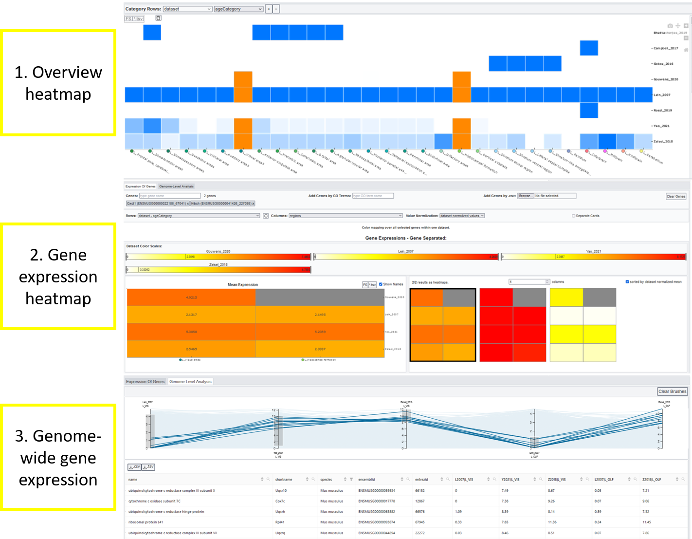
1. Overview heatmap

The general heatmap is the starting point of further investigations: It shows the distribution of image/sample count for datasets (rows) and brain regions (columns). The darker the higher the count, a white element indicates that no data is available for this combination of dataset and brain region. Datasets can be subdivided by the meta data categories age category, cell type, phenotype, genotype, strain or extended annotation. In this case, a row shows the dataset coverage per category groups.

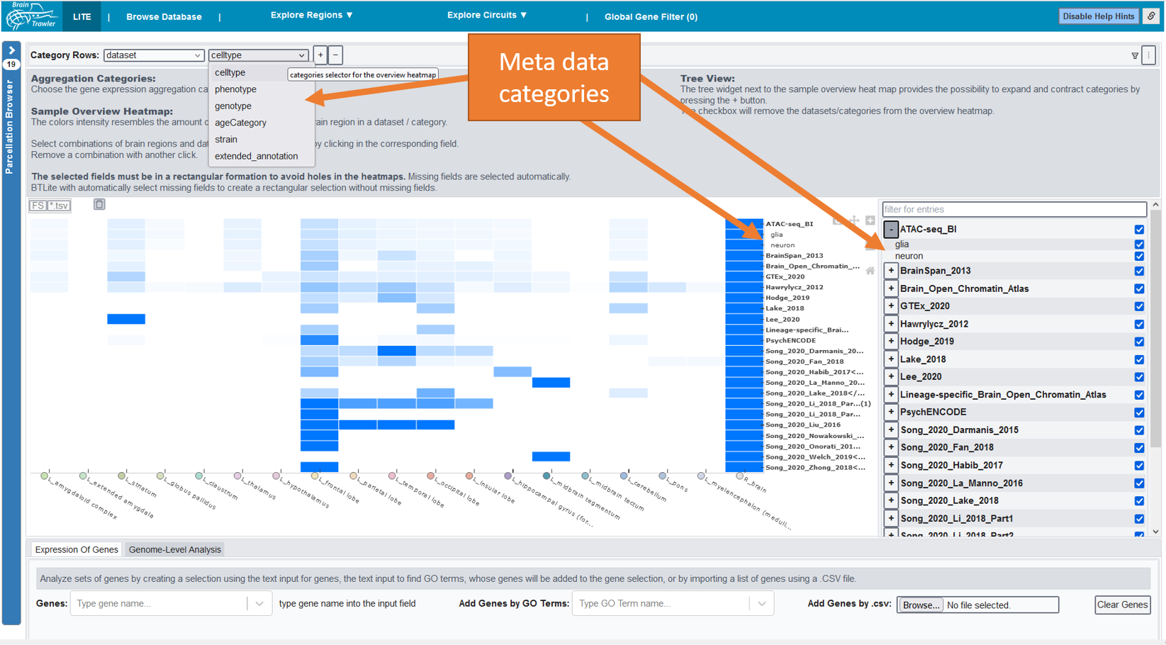
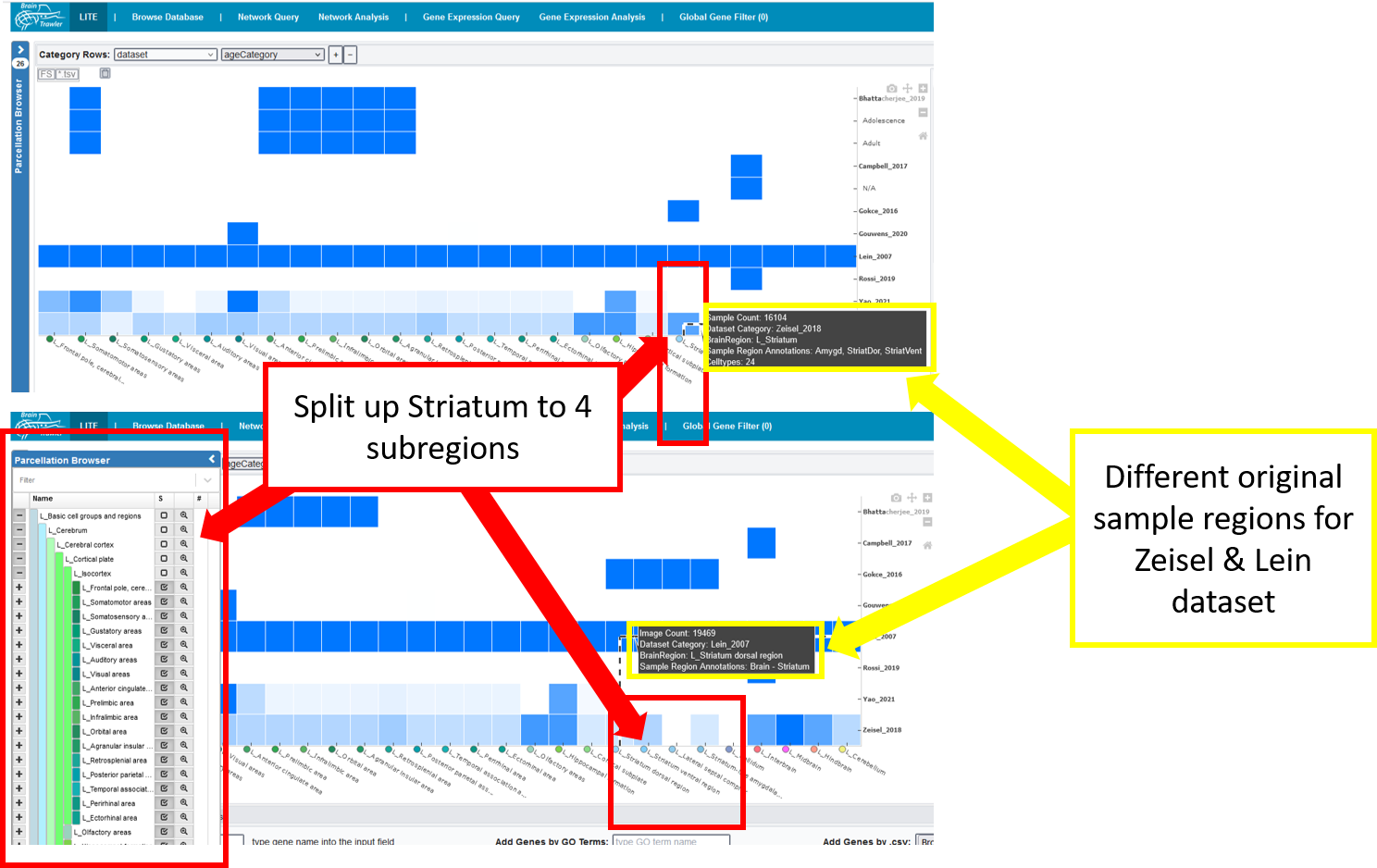
By clicking on the parcellation browser (left side), you can subdivide or merge regions based on the brain ontology. If you hover over an element of your heatmap, you see the current brain region and the original sample region anottation. This information can be used to estimate its relevance for the user. Besides that, you get a summary of the image/sample count, the dataset category = name of the dataset plus maybe a meta data category and the amount of covered meta data categories per category.

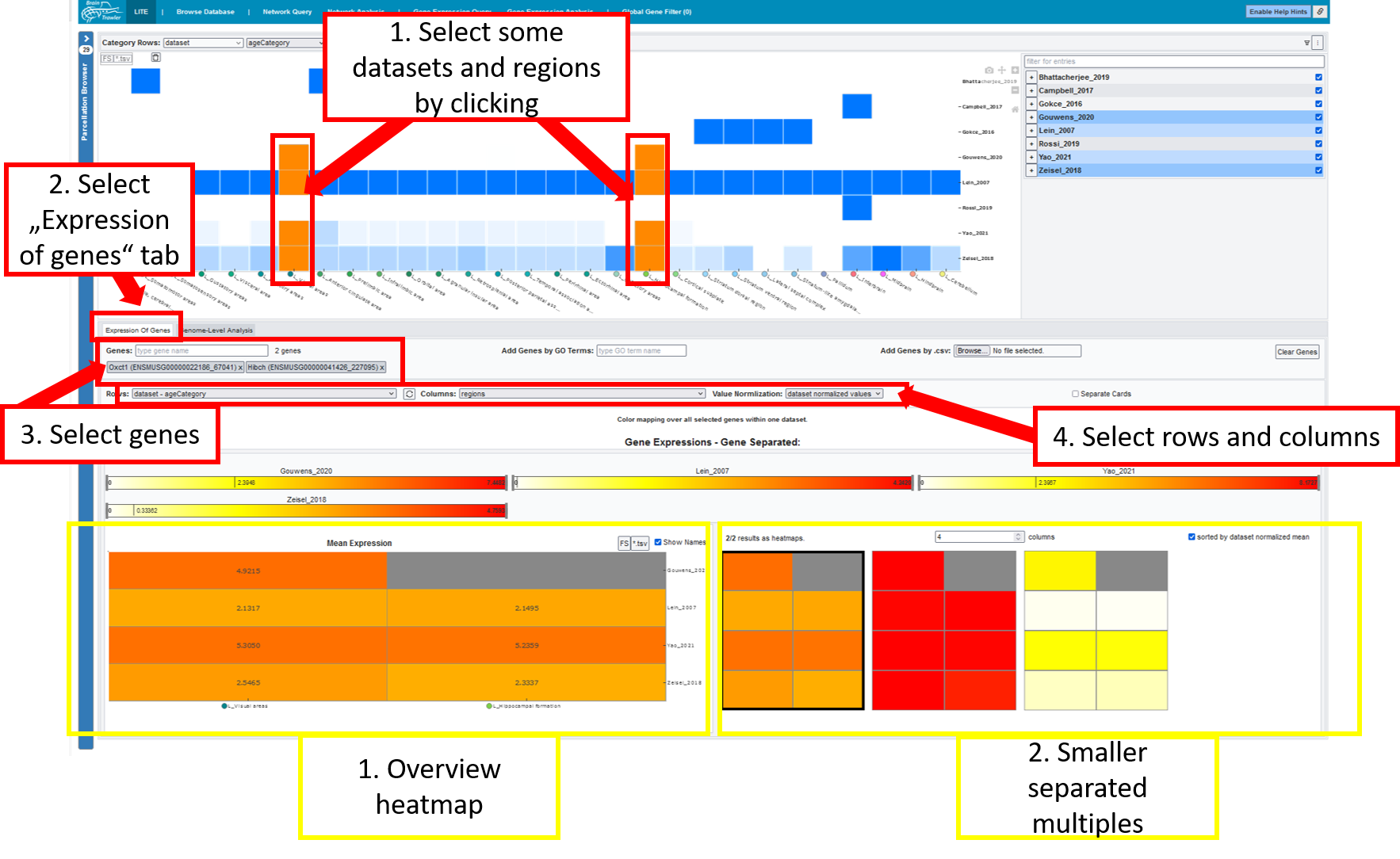
2. Gene expression heatmaps

To investigate the expression of selected genes, you (1) select specific entries of your heatmap by clicking on them, (2) select the “Expression of genes” tab and (3) select some genes. (4) Then you select what your rows and columns should show. Several heatmaps appear, on the left side (1) a big overview heatmap, on the right side (2) small multiples are visalized to see the details. The colours are dataset dependent as the values can’t be compared directly.

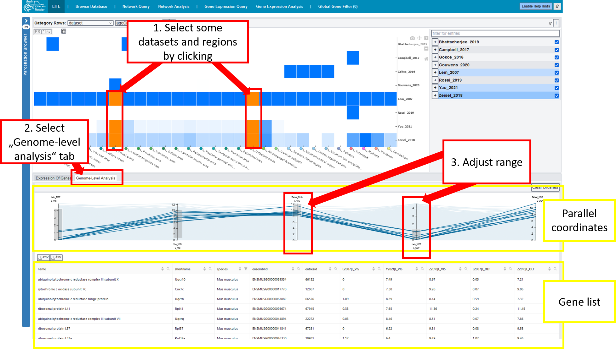
3. Parallel coordinates

To analyse your data on a genome level, you (1) select some datsets and regions by clicking, (2) you select the genome-level analysis tab and then a parallel coordinates system appears. Every line is a gene. (3) For every dataset-region combination you can adjust the range you want to see. You also get a gene list of your filtered genes.

The technical background and more informations can be found in our publication (Ganglberger et al, 2023)

Browse Database

The Browse database tab can be a starting point for all other workflows. Here, one can browse all data in BrainTrawler’s database via a text search or by browsing through the different tabs.

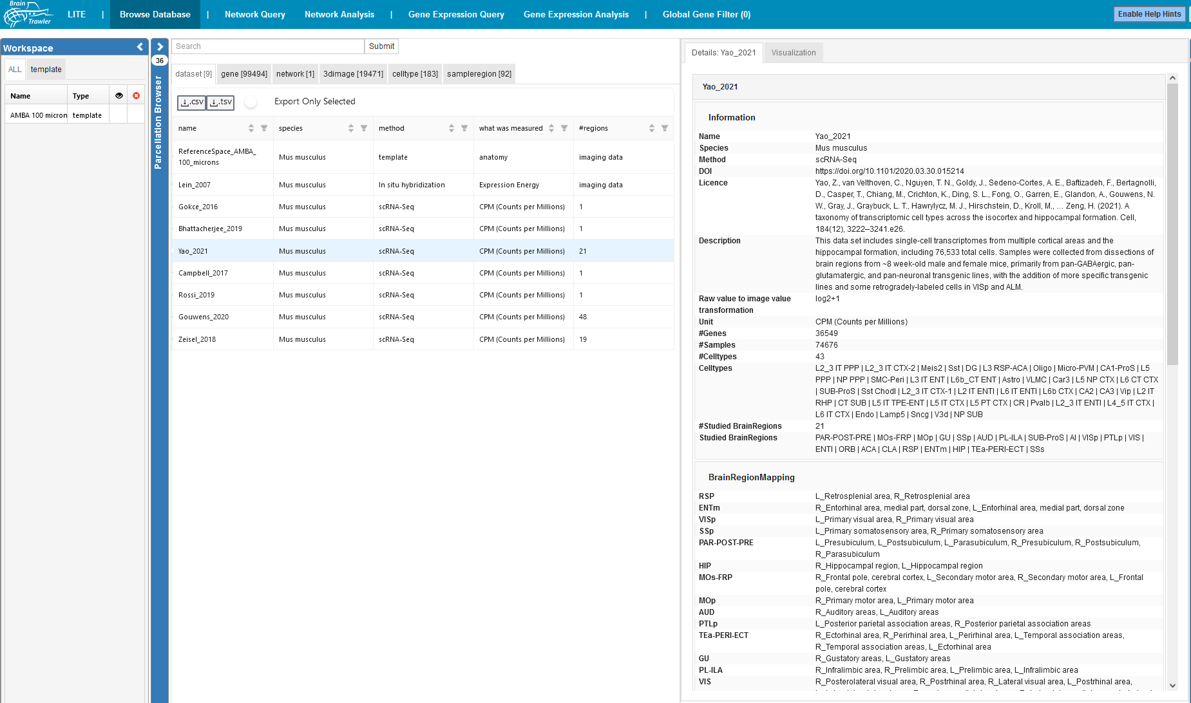
You can see your datasets, genes, networks, 3D images, celltypes and sampleregions. You see some information on the dataset (name, species, method, …). For some items (network and 3D image), it is possible to add/remove them to/from the Workspace List:

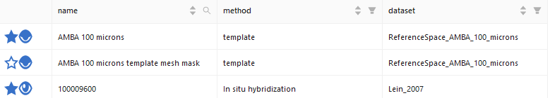
A click on the star icon next to an item adds/removes it to/from the Workspace List. The eye icon next to the star icon will add it to the Workspace too, but also visualizes it directly. This is further indicated by the eye icon in the Workspace List (the eye icons correspond to each other). If the eye icon is active, it means that an item is visualized in the current workflow, and therefore it is in the Viewer Items List. Or simple: Star Icon → Item to Workspace List. Eye Icon → Item to Workspace List and Viewer Items List.

Note

Items that you add as visible to Workspace List (with the eye icon) will be automatically set visible in the Network Query workflow. This is because the Network Query workflow is usually the next workflow after Browse Database, so this saves a few clicks.

Note

Currently only neuron related GO terms are in the database.

RDoC domains

BrainTrawler allows linking of datasets and database circuits to RDoC domains, constructs and sub-constructs. Additionally, free-text keywords can be set for datasets and circuits. For more information on RDoC (Research Domain Criteria) look here.

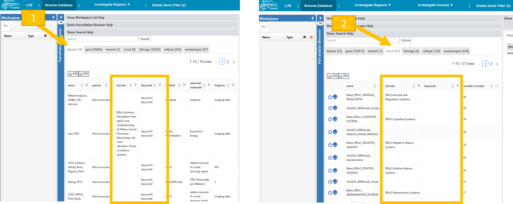
1. Datasets: Go to the “Browse Database” tab, then the subtab for “dataset” is already selected. The displayed table shows for each dataset related RDoC domains, constructs and sub constructs in the column “domain”. The column “keywords” shows free-text keywords for the dataset. These keywords should be set before ingesting a new circuit. Ask the person responsible for data ingestion.

2. Circuits: Go to the “Browse Database” tab, then subtab for “circuits”. The “domain” and “keywords” are there. The database provided by Beam et al. (2021) is integrated, see Circuit database.

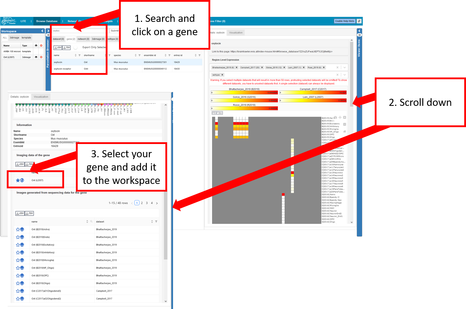
Select gene from Browse Database tab

To add genes from the database to the workspace you do the following:

1. Search for a gene and click on it.

2. Scroll down on the right side until.

3. Select your gene from a dataset and add it to the workspace.

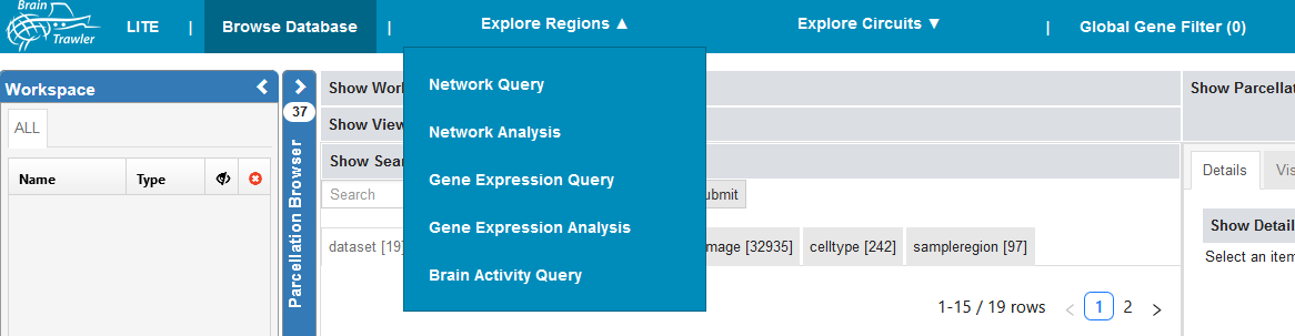
Explore regions

There are several queries and analyses you can perform on brain regions:

1. Nework query & analysis

2. Gene expression query & analysis

3. Brain activity query

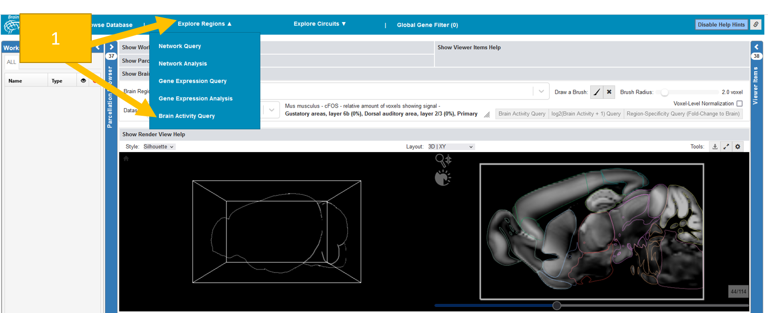
You reach it when clicking on “Explore regions” in the top bar.

The single queries are described in detail in the following:

Network Query

A network query can be conducted in the “Network query” tab.

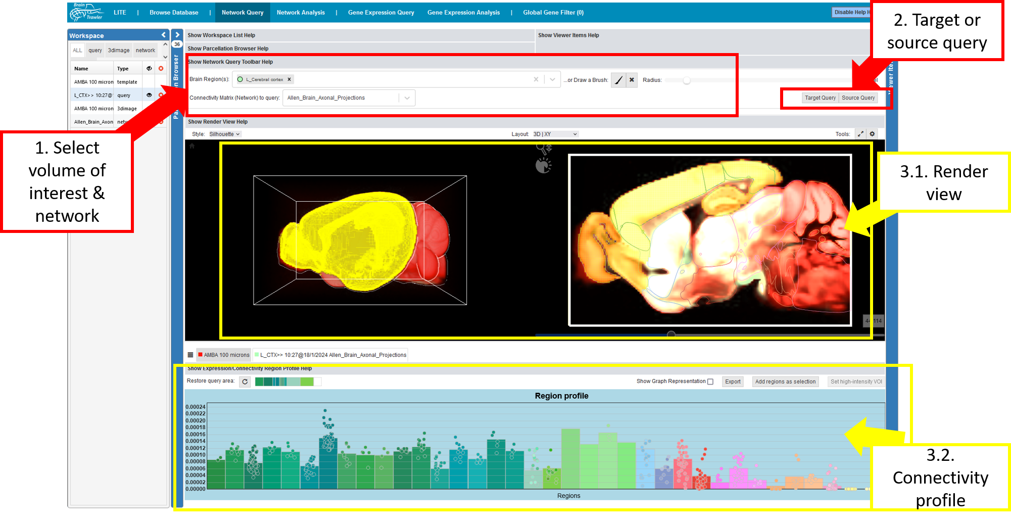
Network queries, such as target or source connectivity queries can be executed as follows:

1. Select a connectivity matrix (network) and a “Volume of Interest” (VOI). This VOI can be one or more brain regions and/or a brush drawing with a certain radius (see also Visual Queries). Brush drawings can be initiated via the “brush” button (initiating a new brush will remove all brushes/selected brain regions). The selected VOI then acts as an input for a target or source query on the selected connectivity matrix (network).

2. Click the “Target Query” or “Source Query” Button, BrainTrawler retrieves the connectivity to all voxels that are either targets or sources from the selection, and then returns a query item (connectivity from/to VOI on voxel-level).

3. The result will be rendered instantly in the

   1. Render View and

   2. as Connectivity Profile. This profile represents the cumulated connectivity to (target) or from (source) the selected VOI. The Query Item gets automatically assigned with the name and color of the largest anatomical brain region in the VOI. Different tabs allow the user to switch between profiles of visible queries/gene expressions.

Afterwards, you can continue and set a high-intensity VOI

High-intensity VOI

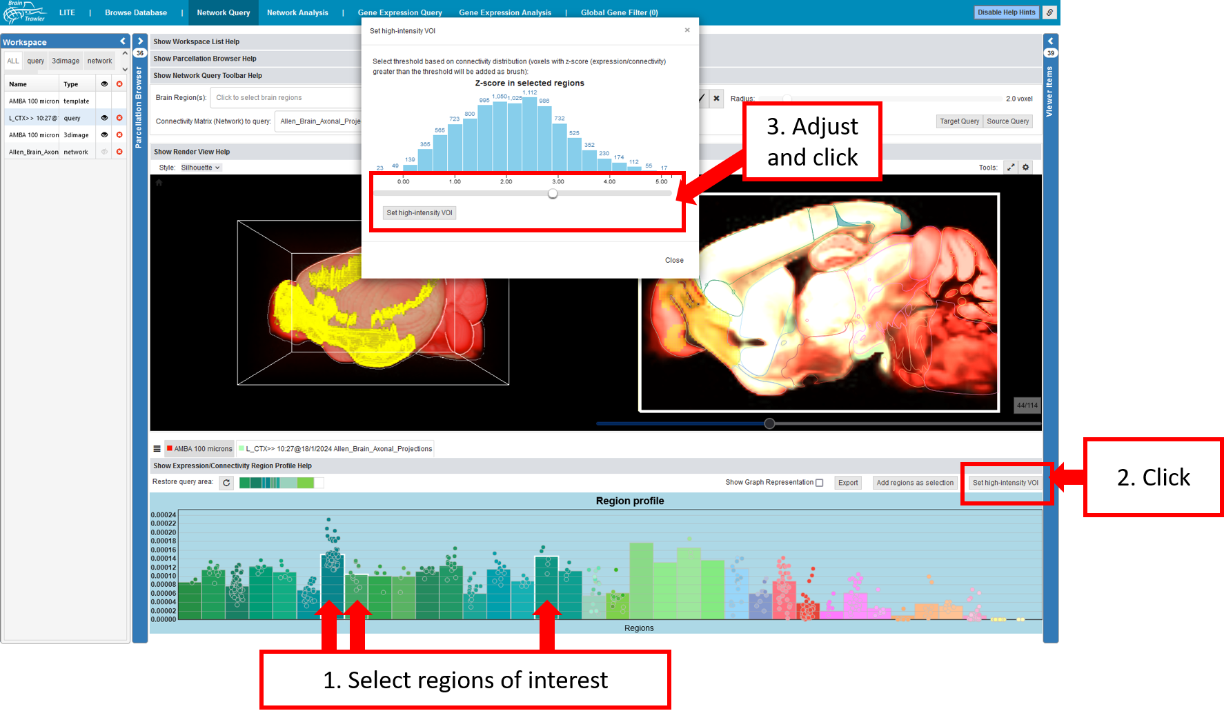
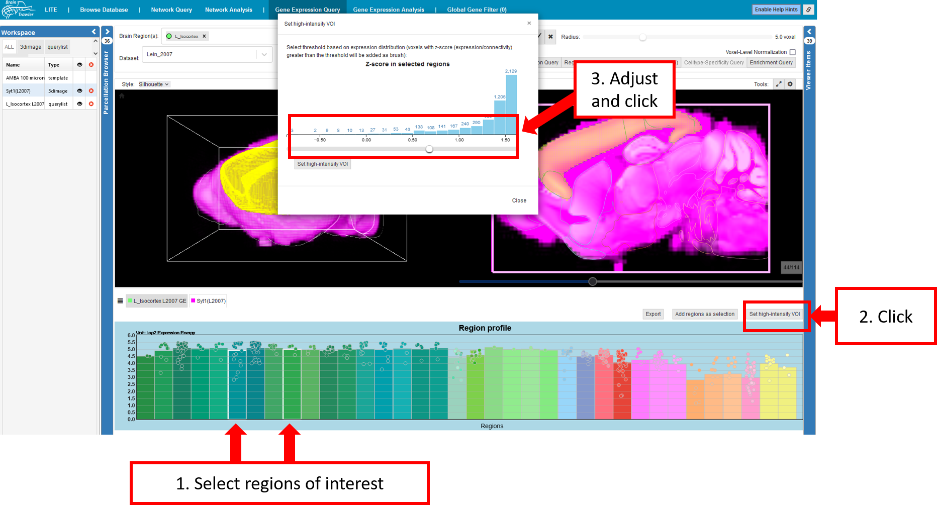
In the connectivity profile (see also Profiles), one can define a VOI with high intensity and do a 2nd order network query:

1. Select regions of interest (e.g. with high connectivity)

2. Click on “Set high-intensity VOI”

3. Choose a threshold in the voxel-level connectivity histogram pop-up, which adds all voxels within the region, and a connectivity above the threshold, as VOI.

Afterwards, you can perform a target/source query on the selection, the resulting second-order connectivity is visualized in 2D and 3D, while the associated Connectivity Profile is rendered again in a tab below the Render View.

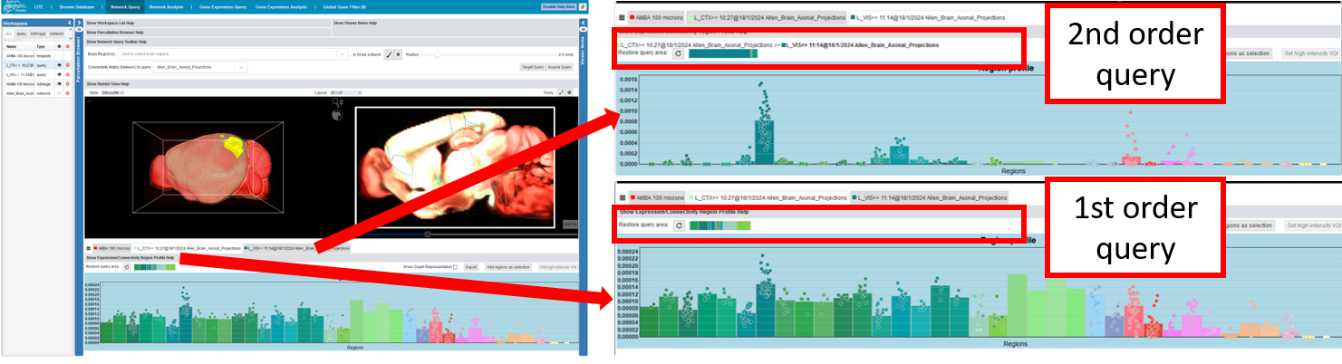
As shown in the figure, one can determine the origin of a 2nd order network query by having a view at the text above the connectivity profile.

An alternative view of the profiles can be rendered by clicking on the “bars” - icon next to the tabs of visible profiles where higher order Connectivity Profiles will be shown below their originating Connectivity Profile.

Typical use case network query

The user selects a structural connectivity matrix in the Query Toolbar, and brushes a VOI in the Render View (for example a region with high gene expression). A click on the “Target Query” button executes the select VOI. The accumulated connectivity is instantly displayed in 3D and 2D and as Connectivity Profile. This process is repeated with a functional connectivity matrix. The user then compares both outgoing connections in the Render View and in the Connectivity Profiles.

Note

Initiating a new brush is (currently) to remove any selection of a VOI that has been made.

Network Analysis

To analyse single networks or to compare multiple ones, you go to the “Network analysis” tab.

Local connectivity (query items, as a result of the Network Query worflow) or global whole-brain connectivity (a network item directly visualized) can be analyzed and compared as region-level networks on different anatomical scales. Instead of the Query Toolbar in the Network Query workflow, it shows information and settings for the network visualization.

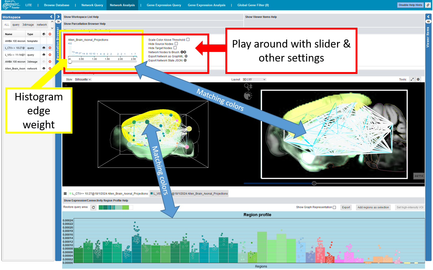
For every visible network item, a histogram of its edges weights shown. The colors of the histogram bars map directly to the visualized edges and can be set in the Viewer Items List. The color directly relates to connectivity strength. Since the number of edges increases quadratically with the number of nodes, one can apply thresholding on edges to hide weaker connections: The threshold can be set with the slider below the histogram.

There are also some further settings:

Scale Color Above Threshold: one can scale the color between the theshold and the maximum value.

Hide Source Nodes and Hide Target Nodes further allows to hide source or target nodes of a network if one wants to focus on these individual parts.

Network Nodes to Brush adds the voxels of all visible nodes of the network to the selection for a Visual Query.

There is also the possibility of a comparison and joint exploration of multiple graphs , which relate to the same anatomical parcellation. This has been realized by overlaying several graphs, i.e. simply rendering multiple edges between nodes. Since showing only two graphs even renders up to four arrows between nodes, one can use an overlap visualization (“Visualize Overlap” checkbox) to emphasize on connections that are strong in multiple networks. Here, only a maximum of two edges per node needs to be rendered (i.e. two for directed, one for undirected). Their weights are defined by the multiplication of all edges (at regionlevel) between those nodes. Unlike an overlap that is based on the presence of connections (i.e. it renders binary edge weights if they are above certain thresholds in different networks), it provides edge weights on a continuous scale to visualize contrast between weak/strong connections. If an overlap is computed, the histograms depict a formula of the multiplication of individual graphs. Cascading queries are treated as a single network, depicted by brackets in the formula , since they represent connectivity of different orders.

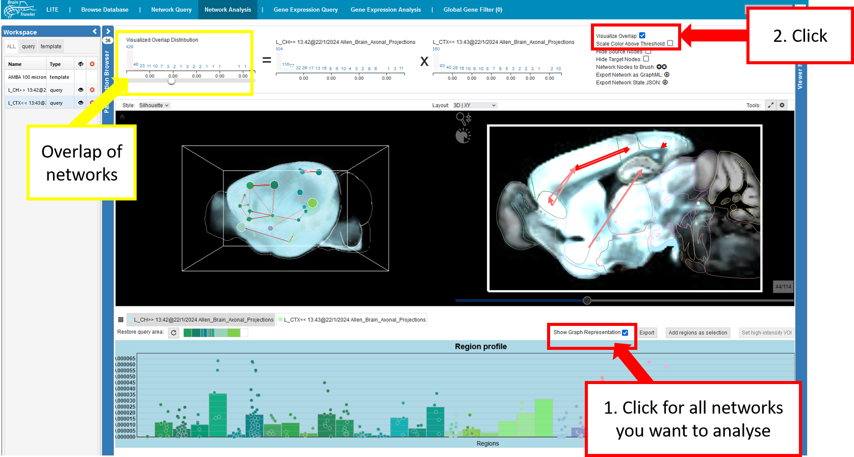
So, summed up, to compare networks you have to:

1. Click “show graph representation” for the networks you want to compare

2. Click “visualize overlap”

Then, you can play around with your network as before.

Note

Query items from the Network Query worflow will be automatically set visible in the Network Analysis workflow. This is because the Network Analysis workflow is usually the next workflow after Network Query, so this saves a few clicks.

Gene Expression Query

Gene Expression Queries can be performed to see which genes are specific for certain brain regions. The workflow is similar to a Network Query. There are multiple explorative queries and a differential gene expression analysis (DGEA) available:

Explorative Queries

You reach the explorative queries under

1. To get to the query tab:

1. Navigate to “Explore Regions”, then to “Gene Expression Query”

2. Select the “Query Gene Expression Analysis” subtab.

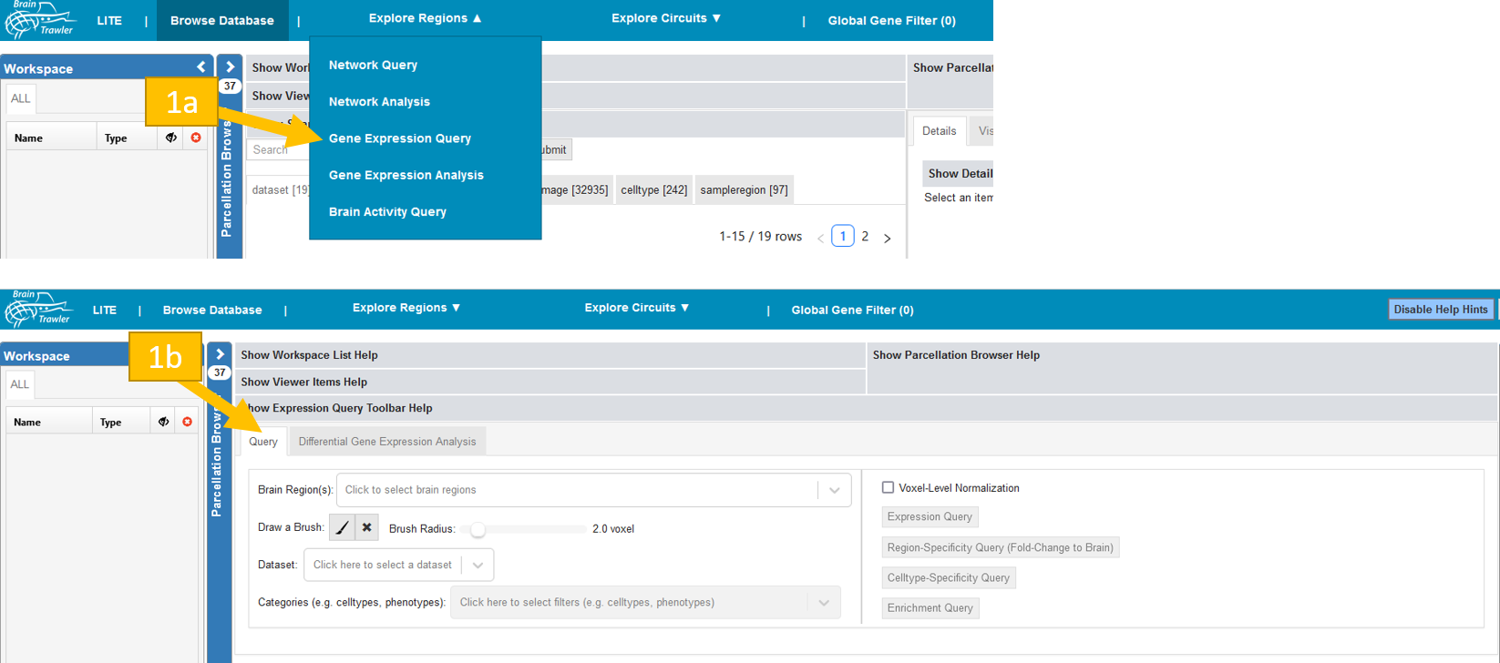
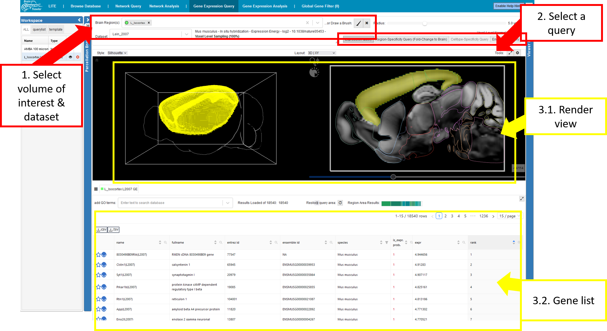
For a query do the following:

1. Select a dataset and a “Volume of Interest” (VOI). This VOI can be one or more brain regions and/or a brush drawing with a certain radius (see also Visual Queries). Brush drawings can be initiated via the “brush” button (initiating a new brush will remove all brushes/selected brain regions). The selected VOI then acts as an input for the gene expression query.

2. Select one of the four available queries Expression query, Region-Specificity query, celltype-specificity query, Enrichment query. More details are given below.

3. The result will be rendered instantly in the

   1. Render View and

   2. as a Gene list giving the name of the gene (name, fullname and entrez id), the species, the probability of being expressed, the value of the expression and the rank.

There are four different types of Gene Expression Queries that represent different types of normalization:

• Expression Query: Genes ranked by their mean gene expression within the VOI (for example: in case of the Allen Mouse Brain Atlas: expression energy)

• Fold-Change to Brain Query: We compute the fold-change to the rest of the brain: mean gene expression within the VOI DIVIDED by the mean gene expression of the whole brain.

• Celltype-Specificity Query: This query can be used to see how specific the expression of a certain celltype is. Note that this query makes only sense, if a filter based on a celltype is applied. In this case, the mean gene expression within the VOI (similar to the Expression Query) is computed, and normalized by the expression over all celltypes (filters not concerning the celltype are still applied): mean expression in the brushed region DIVIDED by the mean expression of the brushed region for all celltypes.

• Enrichment Query: Generalization of celltype-specificity query. This query can be used to see how specific the expression of the selected filter categories is. Note that this query makes only sense, if a filter is applied! In this case, the mean gene expression within the VOI (similar to the Expression Query) is computed for all samples of the selected filter/categories, and normalized by the expression over all samples (filters not applied): mean expression in the brushed region for the filter/categories DIVIDED by the mean expression of the brushed region for all samples.

Note

The Gene Lists contain only genes with expression/specificity>0! That’s why the do not always show all genes in the database.

Note

If datasets do not span the whole brain, z-score has been computed for the regions of the respective dataset (and not the whole brain).

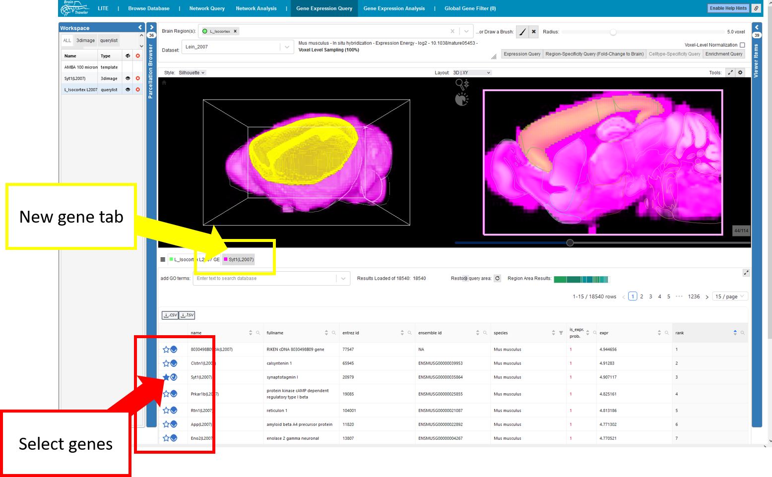
You can view genes and select them to the workspace by clicking on the eye/star icon in the gene list. That way a new tab for the gene appears.

Then, similar to Network Query second order queries can be done based on high intensity VOI:

Differential Gene Expression Analysis (DGEA)

A differential gene expression analysis (DGEA) based on t-tests with FDR correction is now possible in BrainTrawler.

Note

Differential gene expression analysis in BrainTrawler is based on t-tests, which require a normal distribution of gene expression values. This assumption might not always be fulfilled. Therefore, this feature should only be used for hypothesis generation and results obtained here should be validated further.

1. To get to the query tab:

1. Navigate to “Explore Regions”, then to “Gene Expression Query”

2. Select the “Differential Gene Expression Analysis” subtab.

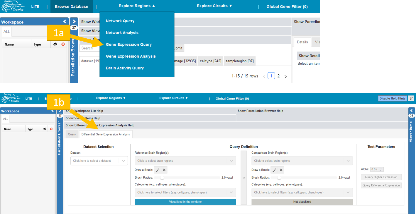
2. To perform the DGEA: Select a dataset in the block “Dataset Selection”. Afterwards in the block “Query Definition” choose a region and (if you want) categories for filtering for reference and comparison. Whether reference or comparison region is visualized in the renderer is indicated in blue with the text “Visualized in the renderer” or in grey “Not visualized”. The switch button ⇌ between reference and comparison block can be used to switch reference and comparison definition. Finally, in the block “Test Parameters” choose your level of significance alpha and query for differential or higher expression by clicking on the respective button. The computation could take some time.

Note

In the “dataset selection” block you can see whether your selected regions are part of your dataset. The dataset can either cover the full, parts or not cover the query area. In that case use another region or dataset.

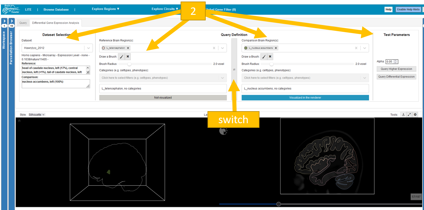
3. As result, a volcano plot and a table where each row corresponds to a gene in the dataset is shown. In the volcano plot, you see for every gene the log2 of the fold change and the log 10 of the q-value. In blue or yellow the down or up regulated genes can be seen. The filters can be applied for the plots and the table. For each gene, its short name, full name, ensembl and entrez id, as well as p-value, q-value and fold change are displayed. Genes are sorted first on q-value and second on fold change if the q-value is the same. There is also a division by zero column: For voxel-level datasets, gene expression values are stored with reduced accuracy for faster performance. This may cause divisions by zero for some calculations required for the differential gene expression analysis. To circumvent divisions by zero, the denominator is set to the lowest positive number possible or a reasonable substitute. Filters for q-value, p-value and fold change are available above the table on the left. A legend above the table on the right gives additional information and also points to Result Help for further information. You can also export the meta information and the filtered table.

Gene Expression Analysis

Gene expression query list items (i.e. lists of genes sorted by gene expression) reveal which genes are specific for a certain VOIs. Since every gene list consists of several thousand genes, an efficient comparison and combined filtering of these lists can be done with a parallel coordinate system.

Note

You have to perform Gene Expression Queries first before you can perform the gene expression analysis in this workflow/tab!

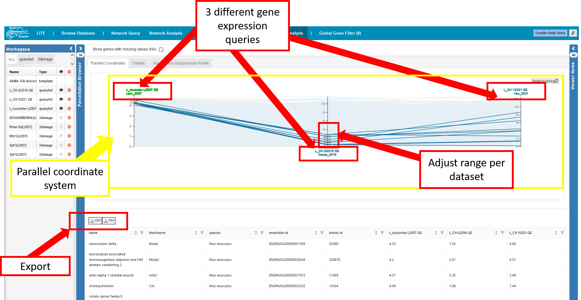
A parallel coordinates system allows the filtering of multiple gene lists from different brain regions by their gene expression. Each axis represents a gene expression query, and as a consequence the gene expression for the query regions (the color of a label indicates the color of largest region in the query’s VOI). Each line represents a gene. A selection/filtering of genes with specific gene expression patterns can be made drawing brushes (the grey boxes) on an axis, you adjust the range per dataset. You can remove the filters with the “Reset Brushing” button (they are also reseted when tabs are switched).

Brushed genes in the parallel coordinate system are automatically filtered for in the table below. The table can be also exported as tsv (tab separated values) with the “.csv”/”.tsv” button of the table.

The parallel coordiantes system and the table below only show genes without missing values (NA), but they can be enabled via the checkbox. In the parallel coordiantes system, missing values will be interpreted as 0.

Note

Query list items from the Gene Expression Query worflow will be automatically set visible in the Gene Expression Analysis workflow. This is because the Gene Expression Analysis workflow is usually the next workflow after Gene Expression Query, so this saves a few clicks.

Brain Activity Query

Brain Activity Queries can be performed to see which fMRI subjects show brain activity in certain brain regions (cFos imaging also available). Similarly to Gene Expression Queries, they can be executed from VOIs (Volume of Interest) selected by brush or brain regions. A Brain Activity Query query retrieves the the mean brain activity of the VOI for every subject, and renders it instantly as filterable Subject List below the Render View in a tab similar to Expression/Connectivity Profiles.

1. Go to Explore regions and select Brain activity query.

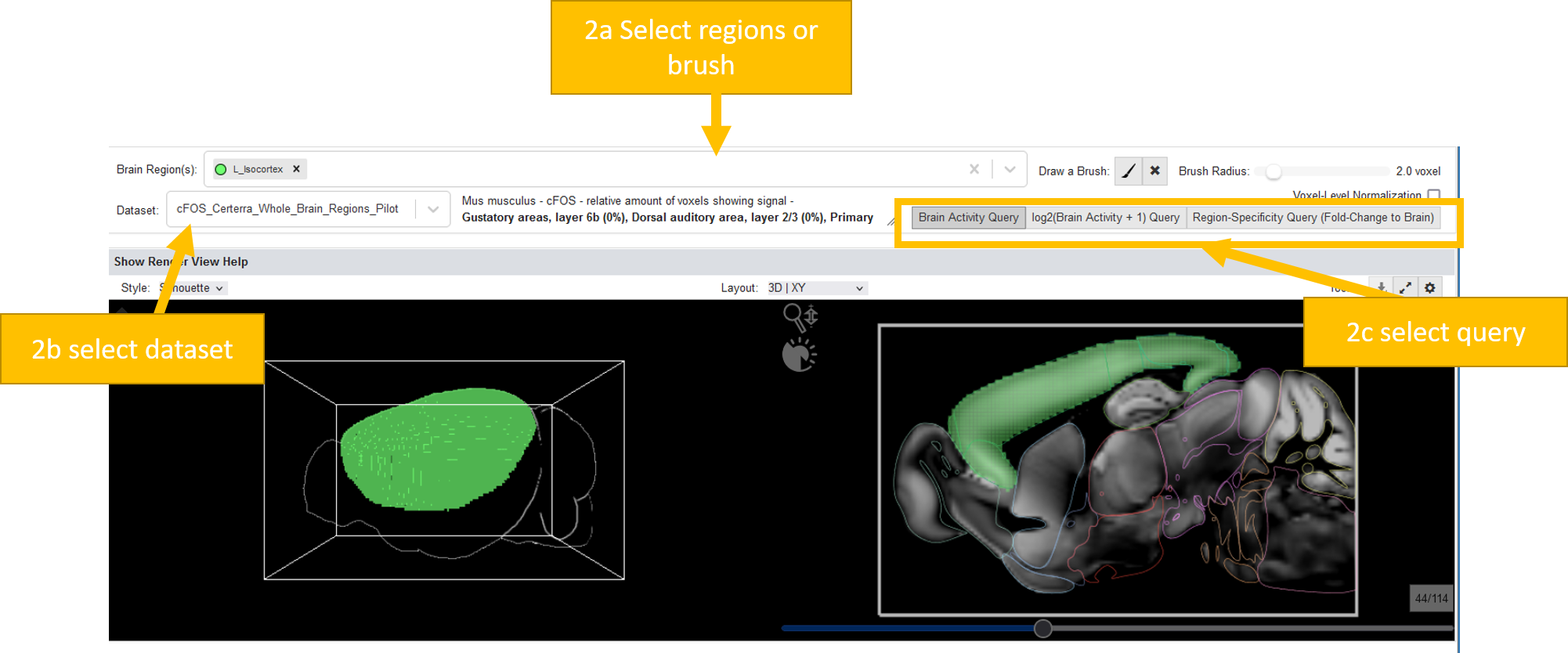
2. Querying a brain activity dataset works exactly like querying a gene expression dataset:

1. Make a spatial selection (either by selecting a brain region or by brushing)

2. Select a dataset

3. You can select from three query types:

• Brain Activity Query: Returns a list of subjects ranked by their mean brain activity in the brushed region

• log2(Brain Activity + 1) Query: Returns a list of subjects ranked by their mean log2(activity+1) in the brushed/selected regions. This leads to nicer distributions in the violin plots and a better (is_active) estimation

• Region-Specificity Query: Returns a list of subjects ranked by their specificity for the brushed/selected regions (VOI): Mean brain activity in VOI DIVIDED By mean brain activity over the whole brain (=fold change to brain).

3. You will retrieve below:

1. violin plots of your results and

2. a table showing the subject images, ordered by their activity/region specificity in the selected region

4. To visualize the activity in a subject, add it to the renderer and the workspace by clicking the eye-icon

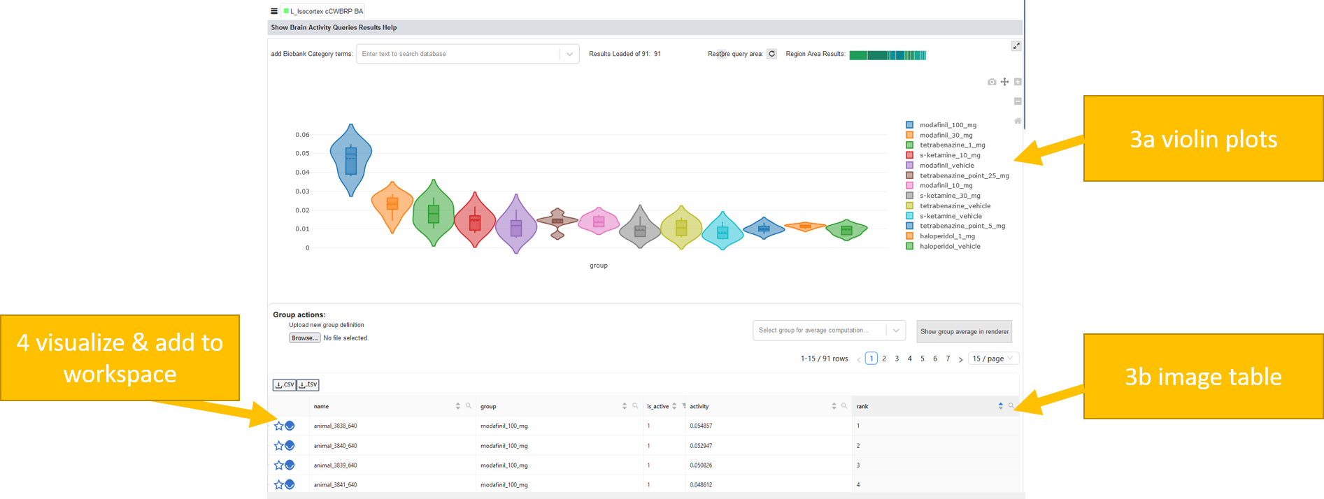
5. Now you could create a circuit from this, as described in Create and edit circuits

Note

You can enable/disable voxel-level normalization. Here, query results will be normalized based on their ratio covering the query area, e.g. if measurements/samples of a region cover 90% of the query area, they will be weighted 9 times as much as measurements/samples that cover only 10%. This is the case for voxel-level data anyway, so there won’t be a difference for this type of data. On by default to account for the region size of the measurements. The name and color of the resulting Query List item (i.e. in the Workspace List and Viewer Item List) are automatically assigned with the name and color of the largest anatomical brain region within the VOI.

Explore Circuits

BrainTrawler allows you to investigate brain circuits. Circuits consist of several nodes.

Create and edit circuits

BrainTrawler allows creating and editing circuits. You have several options: load from database or file, generate circuits from brain activity images or create your own circuit from brain regions. You can edit existing circuits and save them to a file.

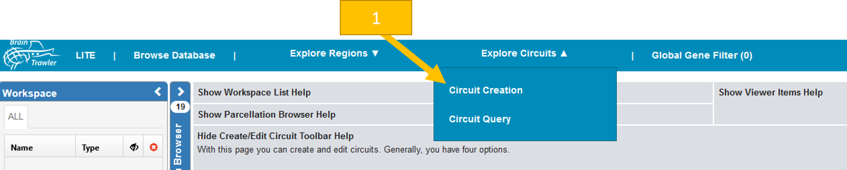
1. You reach the page by clicking in the top bar “Explore circuits” and then “Circuit Creation”.

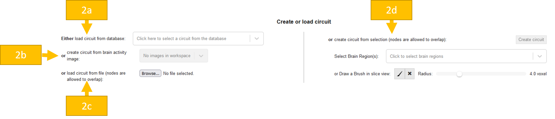
2. Now you have four possibilities to load/create a circuit:

1. Load circuit from database: Click to select one of the circuits in the Circuit database. Currently, only circuits for human are in the database.

2. Generate circuit from brain activity image: The idea is to create a circuit from a brain activity query. One option is to follow the workflow in described in Brain Activity Query. The alternative is to select for a 3dimage of interest in the Browse Database tab by clicking on the star or the eye. Now you can select the image on the create circuits page. You can select a threshold, otherwise, every active voxel will be used. The single nodes are computed by a region growing segmentation: activated areas that are not directly connected with others become a node. Nodes with less or equal 20 voxels are discarded.

3. Load circuit from file: Load a json circuit file from your computer. This could be a circuit you created and saved earlier or a circuit from a colleague. Only circuits of your current species can be used.

4. Generate circuit from selection: select one or multiple brain regions and/or one brush. Then click on the Create circuit button.

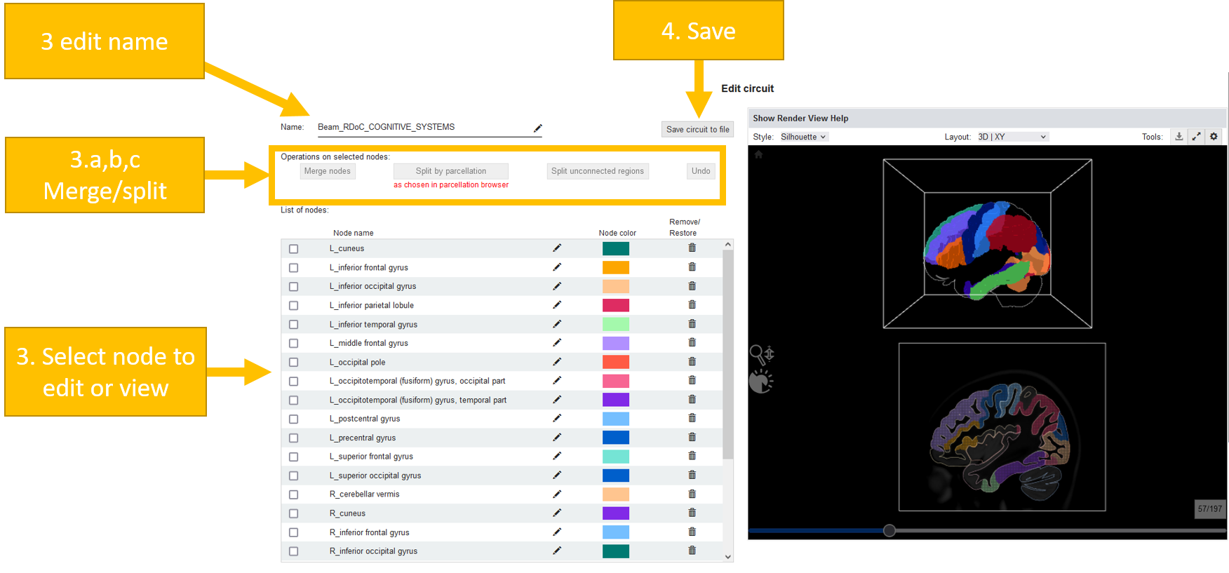
3. Afterwards, you can edit your circuit. First, you maybe want to edit the name of your circuit. You will also see a table containing all of your nodes. Every node has a name, which you can edit. By clicking on the checkbox you can see your node in the renderer with its color. You can merge and split nodes:

1. Merge nodes: You can merge selected nodes to one node. The single nodes are now deleted and only the merged node is available.

2. Split by parcellation: BrainTrawler uses the anatomical Allen Brain Reference Atlases for mouse and human for its brain parcellations. These parcellations organize brain regions hierarchically, meaning that regions can consists of multiple subregions. E.g. assume you have the region Thalamus. This can be divided into dorsal thalamus, epithalamus and ventral thalamus. The level of detail can be selected in the Parcellation Browser (on the left between Workspace and this part of the page, see also help section about it). So in case you have the region Thalamus as a node, but actually you would like to work with the three separate nodes containing its subregions instead, check the level of detail of this region in the Parcellation browser and (if needed) click on the + sign. Now you can click on the button Split by parcellation and your node will be splitted into these three separate nodes.

3. Split unconnected regions: A region growing algorithm is applied and splits the node to multiple nodes in case it contains unconnected areas. Nodes with less or equal 20 voxels are discarded.

4. When your circuit is ready, you can click Save circuit to file and store the json somewhere for later use or send it to a colleague. Now you are ready for a Circuit query!

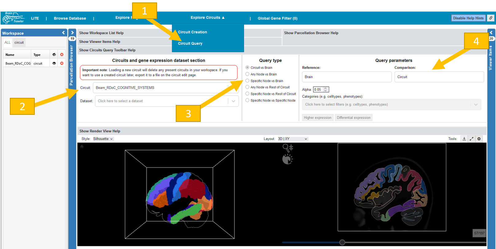
Circuit query

BrainTrawler also allows the investigation of the circuits w.r.t. gene expression based on Differential Gene Expression Analysis (DGEA).

1. Click on “Investigate Circuits” in the top panel and click there on “Circuit query”.

2. Select a circuit and a dataset. Some datasets might not completely cover your circuit. You see a percentage of “Circuit coverage” after selection.

3. Now select a query type. You can do a comparison based on DGEA for:

1. circuit vs brain

2. any circuit node vs brain

3. specific circuit node vs brain

4. any circuit node vs rest of circuit

5. specific node vs rest of circuit

6. specific node vs specific node

4. Now you can select some query parameters. Reference and comparison depend on the query type. So e.g. for “Specific node vs brain” you have to select your node of interest as “Comparison”. You can also define the alpha value. Furthermore, you can filter for categories like cell types, phenotypes etc. You can do either “Higher expression” or “Differential expression” query. For “higher expression”, you do a one-sided test for genes expressed higher for “Comparison” than for “Reference”. A “differential expression” is done via a two-sided test.

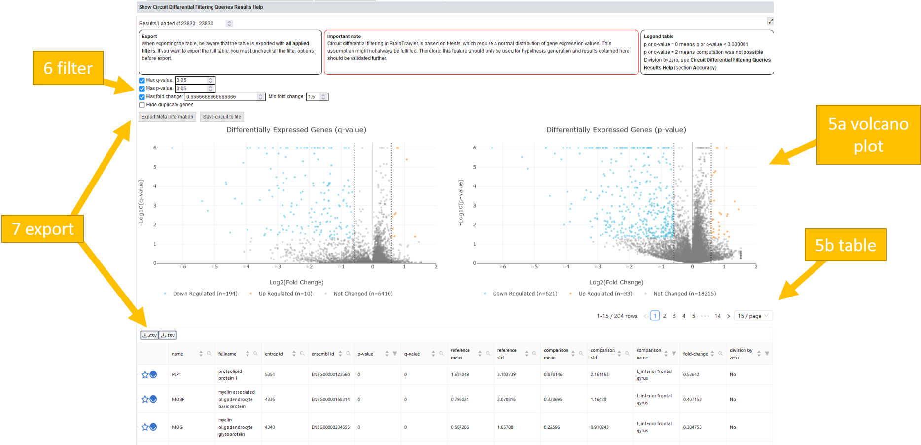
5. The computation might takes some time. Afterwards, a volcano plot and a table will appear below the visualized brain showing your results.

1. In the volcano plot the up and down regulated genes are displayed in blue or yellow.

2. The table will show for every gene the mean and standard deviation of reference and comparison. Furthermore, the fold change is shown. There is also a division by zero column: For voxel-level datasets, gene expression values are stored with reduced accuracy for faster performance. This may cause divisions by zero for some calculations required for the differential gene expression analysis. To circumvent divisions by zero, the denominator is set to the lowest positive number possible or a reasonable substitute.

6. You can also filter by q-value, p-value and fold change.

7. It is possible to export the meta information about the query you did (json) and the filtered result table (csv or tsv).

Note

Differential gene expression analysis in BrainTrawler is based on t-tests, which require a normal distribution of gene expression values. This assumption might not always be fulfilled. Therefore, this feature should only be used for hypothesis generation and results obtained here should be validated further.

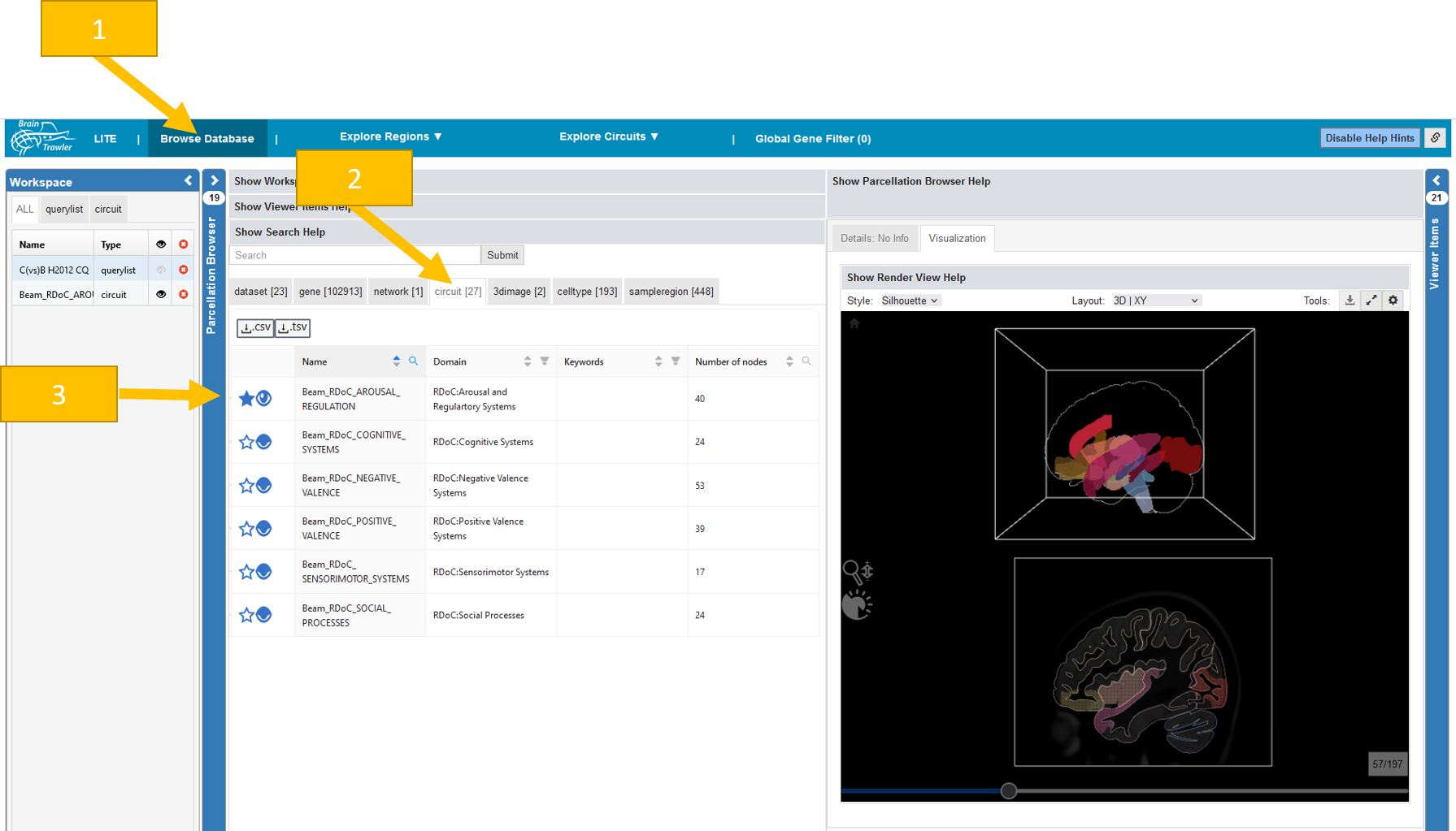
Circuit database

BrainTrawler allows the retrieval of curated circuits from a database. Such database circuits can e.g. be defined based on publications. However, the regions used in the publication need to be matched to BrainTrawler‘s hierarchical parcellation.

To look at the integrated circuits do the following:

1. Navigate to the “Browse database” tab.

2. Select the “circuit” subtab. This will display a list of all available circuits in the database. Currently, only for human circuits are available in the database.

3. By clicking on a row, you see additional information on the circuit on the right. Via the eye icon, you can add a circuit to the workspace and visualize it by changing from “Detail” to “Visualization”. Please note that only one circuit can be loaded and visualized at once.

For the ingested circuits see Circuit data.

A domain expert mapped the regions in the paper to the Allen Human Brain 3D atlas.

Global Gene Filter

In the Global gene filter tab, you can define global gene list filters for all tabs, except for BrainTrawler LITE. All results, no matter if it is the text search in the Browse Database tab/workflow, or results of a Gene Expression Query, will be filtered by the genes you select in the “Globally Used Genes” table. You can either select the genes manually in the table, or upload a gene list (as csv/tsv), containing gene identifier (entrezid, ensemblid, symbols) in a column. These can then be matched with the database.

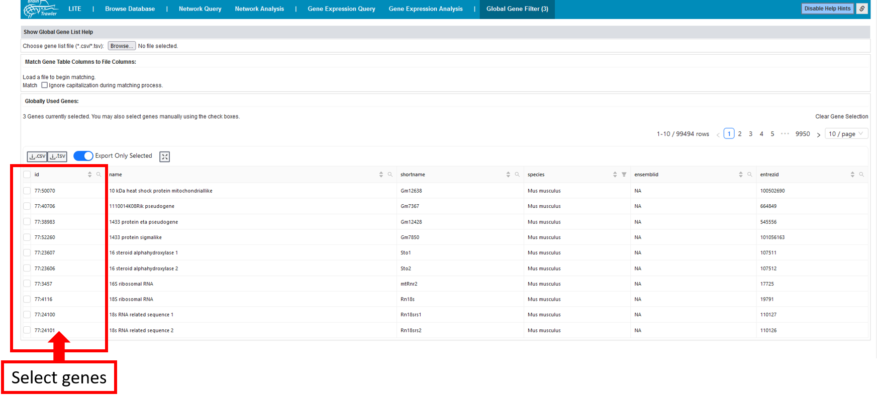
Afterwards, only these selected genes will be displayed, e.g. for a gene expression analysis you have only your (in this case two) selected genes:

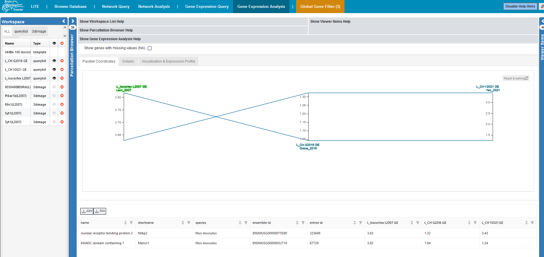
When the global gene filter is active, the tab “Global Fene Filter” is highlighted in orange.